Using the Plugin

Plugin Usage

Click on the tabs below to view the corresponding functionality.

DeskewingQuick DeskewDeconvolutionCroppingWorkflowOutput (Saving files)

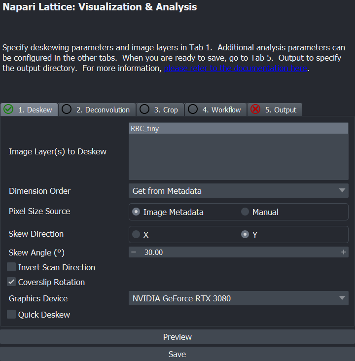
To use the specific image for processing, you will have to select it under the Image Layer(s) to Deskew box on the right. Here, we will click on RBC_tiny. As its a czi file it should read the metadata accordingly and you will see a green tick.

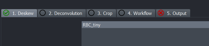
If you are loading a czi, the metadata fields should be populated automatically.

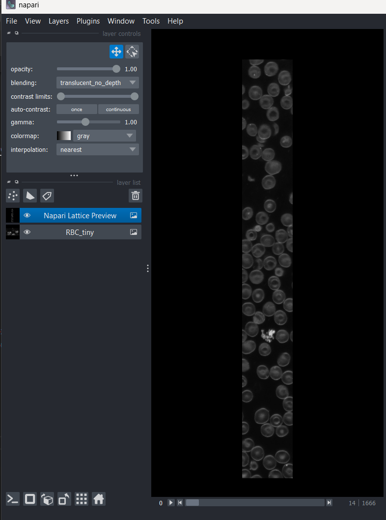
To Preview the deskewed image, click Preview and choose the appropriate channel and time.

You should see the deskewed image appear as an extra layer with the Preview suffix attached to it.

Extra_info

If you look at the terminal after deskew, you should see the settings used and any other metadata associated with the dataset. It is handy for troubleshooting.

The deskew options

The Deskew tab collects every parameter needed to interpret and deskew the raw data. For a Zeiss LLS7 .czi, the metadata fills most of these in for you; for other microscopes you set them to match your acquisition geometry.

Option	What it does	How to set it
Image Layer(s) to Deskew	The napari layer(s) to process.	Select your image. If you have multi-channel images, select them together using Shift+Left Click to process them together.
Stack Along	The axis multiple selected layers are stacked along.	Only relevant when you select several layers (e.g. per-channel layers) — choose Channel or Time.
Dimension Order	How the raw array's axes map to Z/C/T/Y/X.	Get from Metadata for a czi; otherwise set it explicitly (e.g. CZYX).
Pixel Size Source	Whether pixel sizes come from the file or are entered by hand.	Image Metadata for a czi; Manual for formats without metadata (then fill Pixel Sizes: XYZ (µm)).
Skew Direction (X / Y)	The axis the acquisition is skewed along.	Y for the Zeiss LLS7 (default). OPM/SOPi systems may be X or Y — match your scan axis.
Skew Angle (°)	The light-sheet angle.	30° for the Zeiss LLS7. Set to your system's angle (e.g. 45° for the OPM datasets in the manuscript).
Invert Scan Direction	Reverses the plane order along the scan (Z) axis before deskewing.	Leave off for the Zeiss LLS. Tick it if your stage/galvo scans in the opposite direction (common on OPM), which would otherwise mirror the reconstruction.
Coverslip Rotation	Whether to rotate the deskewed volume by the skew angle (standard deskew).	On for the Zeiss LLS7 (coverslip-level output). Off for OPM/SOPi to deskew into the shear-only, coverslip-level frame.
Graphics Device	The GPU used for processing.	Pick your GPU (a CPU OpenCL device also works, but slower).
Quick Deskew	Live in-canvas preview of the deskew without processing.	See the Quick Deskew tab.

Choosing settings by geometry

• Zeiss LLS7 — Skew Direction = Y, Skew Angle = 30, Coverslip Rotation = on, Invert Scan Direction = off. A czi populates these automatically.
• Oblique plane / SOPi (OPM) — typically a different Skew Angle (e.g. 45°), manually entered voxel sizes, Coverslip Rotation = off, and often Invert Scan Direction = on (opposite scan direction). See --no-coverslip-rotation.

From version 1.0.3 onwards, we have an option to show the Deskewed image without actually deskewing it. It does not create a new image, but simply transforms the image in the canvas to a deskewed image. This can be useful for quick preview of the data and especially if you have a large dataset that you don't want to process yet.

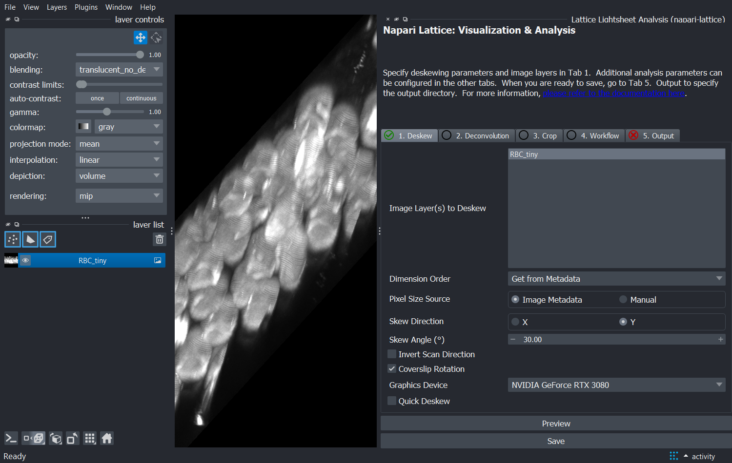
Load and select your image in the Deskew tab, switch napari to 3D view (the cube icon, bottom-left), then tick Quick Deskew at the bottom of the Deskew tab.

Before enabling it, the raw volume is shown skewed — tilted at the light-sheet angle (note Quick Deskew is unticked in the Deskew tab):

With Quick Deskew ticked, the same layer is transformed in-canvas to its deskewed shape, without generating a new image:

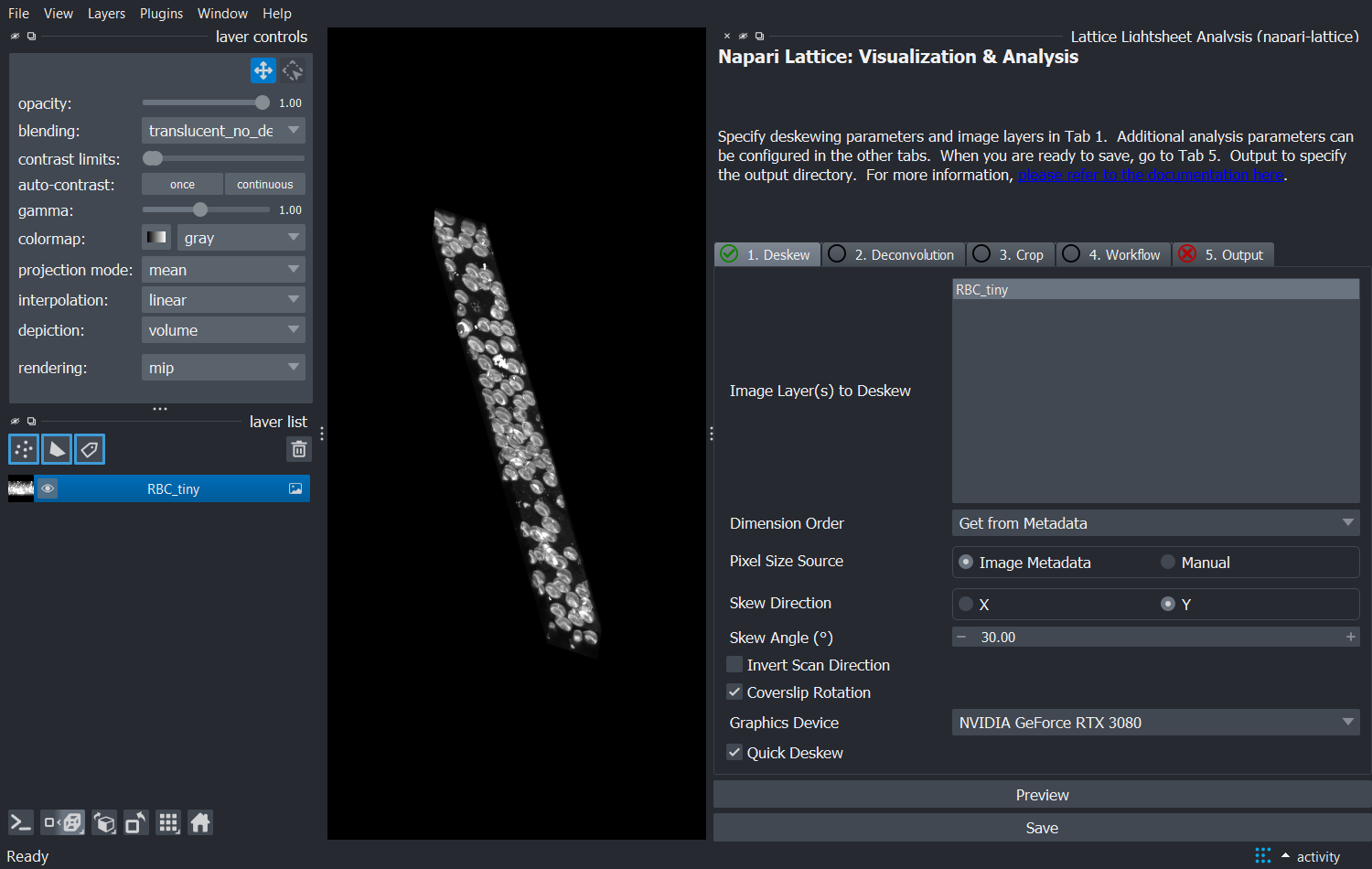
You may get the following warning: Non-orthogonal slicing is being requested, but is not fully supported. Data is displayed without applying an out-of-slice rotation or shear component.! This is absolutely fine. It just means the image won't be displayed as deskewed in 2D mode. Hence, why we enable 3D mode.

Here is an example of browsing through a timeseries

The smoothness of this interactivity will depend on the storage read/write speeds and/or network speeds. For example, if the data is stored on the network, it will be slow to browse timepoints. However, if your data is on your SSD locally, the experience will be much better.

Deconvolution is primarily enabled by pycudadecon. For this functionality, you will need the point spread function (PSF) for the corresponding channel, either simulated or experimentally derived. You can find examples here.

Important

Ensure you are using the right PSF file for each channel. The number and order of the PSF files should match the channels in the image.

After loading the image and configuring it in the Deskew tab, select the Deconvolution tab. When you click Enable, you should see a green tick appear next to the name.

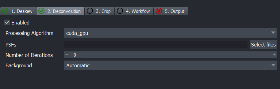
Under processing algorithms only cuda_gpu and cpu are supported. opencl_gpu has not been implemented yet. The next step is to select the PSF files. In this example, we will use the RBC_tiny.czi file

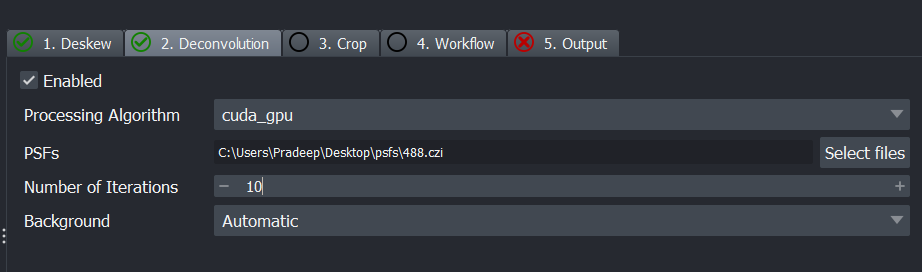
• PSFs: Use the Select files to select multiple PSF files. As the dataset was acquired in the 488 nm channel, we use the 488.czi PSF file here.
• Number of iterations: Try 10 if not sure and increase if needed.
• Background: Background to subtract.
  • Automatic: median value of last Z slice will be used
  • Second Last: median value of second last Z slice will be used. This is used in case the last Z slice is incomplete if acquisition is prematurely stopped.
  • Custom: Enter a custom value

Once you are done, click Preview at the bottom, and select timepoint or channel. You should see output from pycudadecon printed to the terminal. When complete, a deconvolved image will appear as an extra image layer. Below is an example of the deskewed image without (left) and with (right) deconvolution.

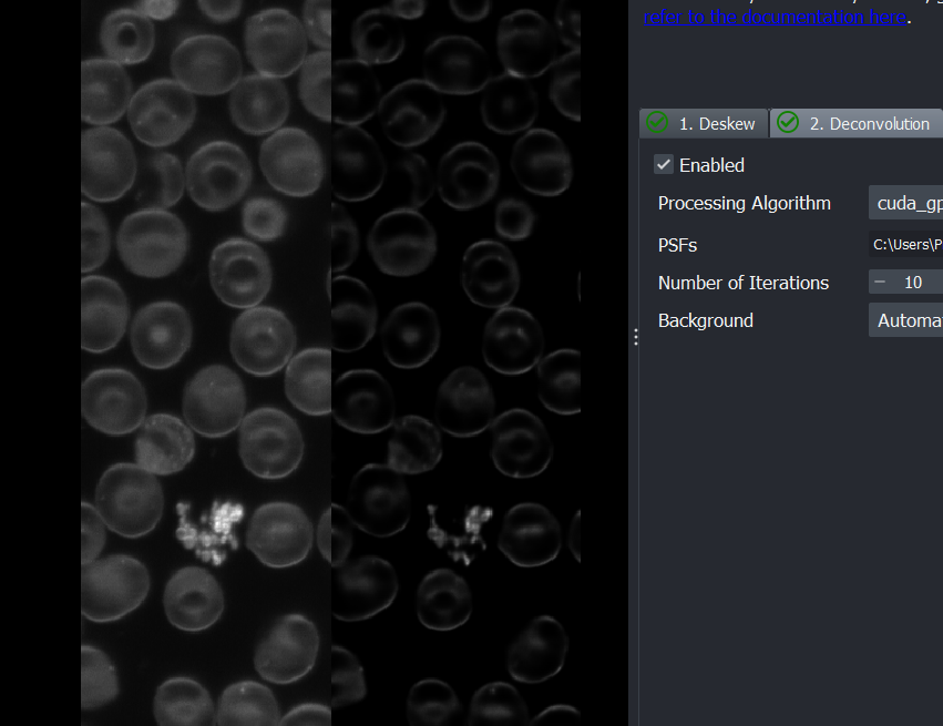
There are two ways to do the cropping:

• Define ROIs within napari-lattice plugin
• Import ROIs generated elsewhere, such as Fiji ROI Manager.

Define ROIs in napari-lattice

• Load and configure the image in the Deskew tab and you should see a green tick.
• Run Preview to get a deskewed volume. We will use this as a reference to draw ROIs for cropping.
• Go to the Crop tab and tick the Enabled button to activate cropping.

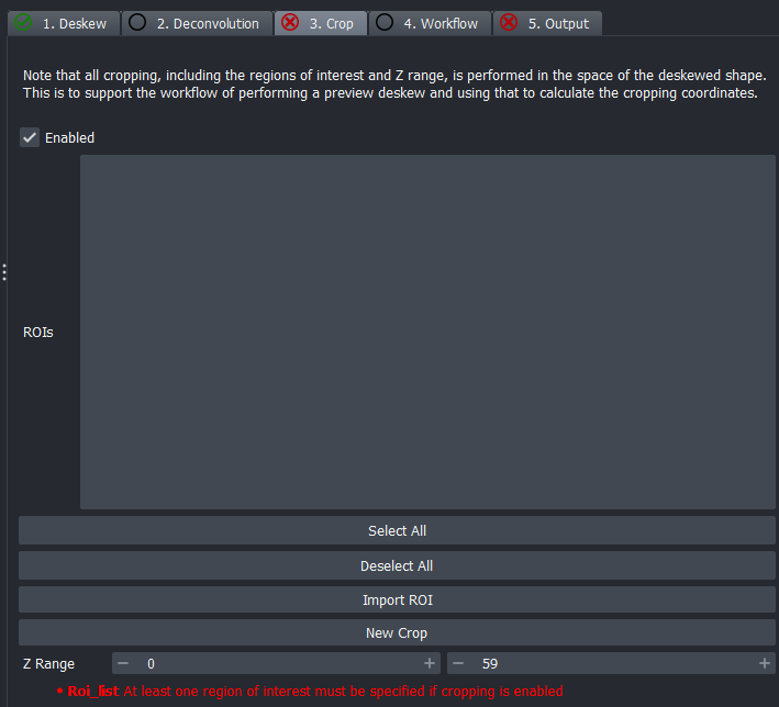
The red text at the bottom indicates that atleast one ROI must be specified.

• Click on New Crop at the bottom of the plugin to add a Shapes layer on the left to draw ROIs. This Shapes layer will be called Napari Lattice Crop. Click here for more info on using Shapes layers and drawing shapes.
• Click on the Napari Lattice Crop Shapes layer and the rectangular ROI tool will be selected by default.
• Draw an ROI around the region you would like to crop. After defining the ROI, it will appear on the right.
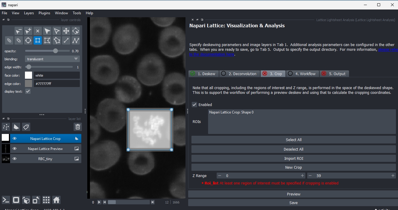
• Similarly, you can draw multiple ROIs. Each ROI will be an entry in the ROIs box. When you select one of them, the error message below will disappear.

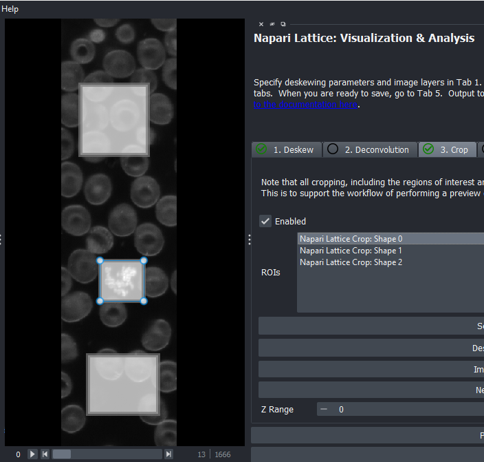
• Once you have drawn the ROIs, select one of them, and click Preview to visualize the cropped region. The cropped image will appear as a new layer in the image layer list on the left.

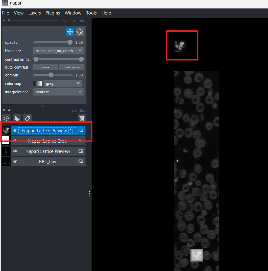
• The purpose of the Crop tab is to setup the ROIs. Once you've defined all of them, you can save all of them by configuring it in the Output tab.

Import ROIs

ROIs can be imported from two file types:

• Fiji ROI Manager files (a .zip, or a single .roi). This workflow exists because the Zeiss lattice lightsheet produces a 2D maximum intensity projection at the end of the acquisition, which can be used to select ROIs of interest in Fiji. Refer to this page for instructions on how to generate and rotate these ROIs. If you do not have an LLS7 MIP, the MIP walkthrough shows how to generate one and turn it into ROIs end to end.
• napari shapes files (.csv), as written by File -> Save Selected Layers. This lets you draw crops now, save them, and reload them in a later session — see Saving ROIs from napari.

To import:

• Configure your image in the Deskew tab (green tick) and go to the Crop tab with Enabled ticked.
• Click Import ROI at the bottom of the plugin and select your ROI file.

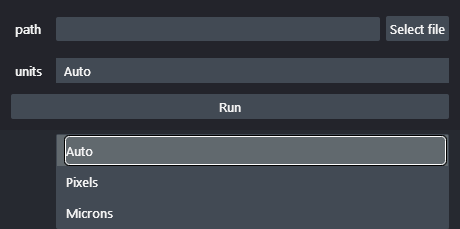
• Leave units on Auto unless you know otherwise (see below).
• The imported regions are added to the canvas as a new Shapes layer with yellow outlines. They are converted into the deskewed image space automatically.
• Select an ROI and click Preview to check the cropped region, exactly as with ROIs drawn by hand.

ROI coordinates and the units setting

ROIs are always interpreted in the space of the deskewed image, so make sure the ROIs were defined against the LLS7 MIP (and rotated as described in Supporting Resources) before importing.

ROI files do not record whether their coordinates are pixels or microns, and the two differ by the pixel size — so Auto decides from the file type: Fiji .roi/.zip are pixels, and a napari .csv saved from a crop layer is microns. Change units only for a .csv written by something other than napari. Getting it wrong scales every ROI by the pixel size, which can still land inside the image, so nothing may look obviously wrong — check the crop Preview before saving.

The conversion uses the pixel size from the Deskew tab, so a manual pixel size set there is applied to imported ROIs too.

The Workflow tab lets you attach a custom napari-workflows analysis pipeline that runs on each deskewed (and optionally cropped/deconvolved) 3D volume. For details on building a workflow, see Workflows.

• Tick Enabled to activate the tab (you should see a green tick).
• Choose a Workflow Source:
  • Active Workflow: use the workflow currently loaded in napari (for example, one you built live with napari-assistant).
  • Custom Path: load a workflow from a saved .yml file. A Workflow Path field appears — select your file.

Info

Whichever source you use, the first step of the workflow must take deskewed_image as its input. See Building a Workflow for how this is defined.

Example: applying a workflow to RBC_tiny

The repository ships some ready-made workflows under workflow_examples/. We will use the single-channel regionprops_workflow, which smooths the deskewed image, segments it with a Voronoi-Otsu labelling, and measures region properties.

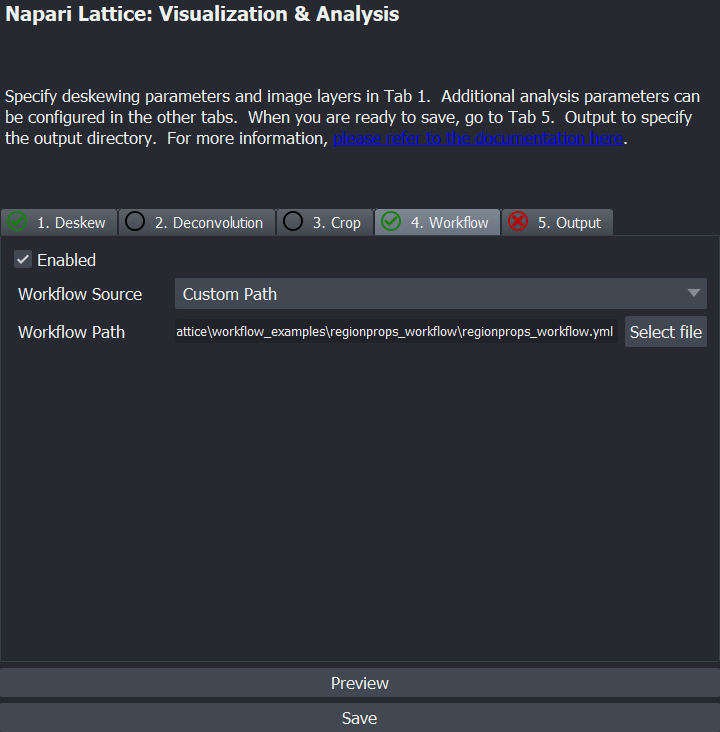
1. Load and configure RBC_tiny.czi in the Deskew tab (green tick).
2. Go to the Workflow tab and tick Enabled.
3. Set Workflow Source to Custom Path.
4. For Workflow Path, select workflow_examples/regionprops_workflow/regionprops_workflow.yml. When the workflow loads successfully, the 4. Workflow tab shows a green tick.

Info

The custom functions a workflow uses (here measure_regionprops.py) must sit in the same folder as the .yml file — napari-lattice imports them automatically when the workflow is loaded.

1. Configure a Save Directory in the Output tab and click Save.

napari-lattice deskews RBC_tiny, runs the workflow on the deskewed volume, and writes the result. This workflow produces a label image (the segmented objects) and a table of measurements — one row per object, per timepoint and channel:

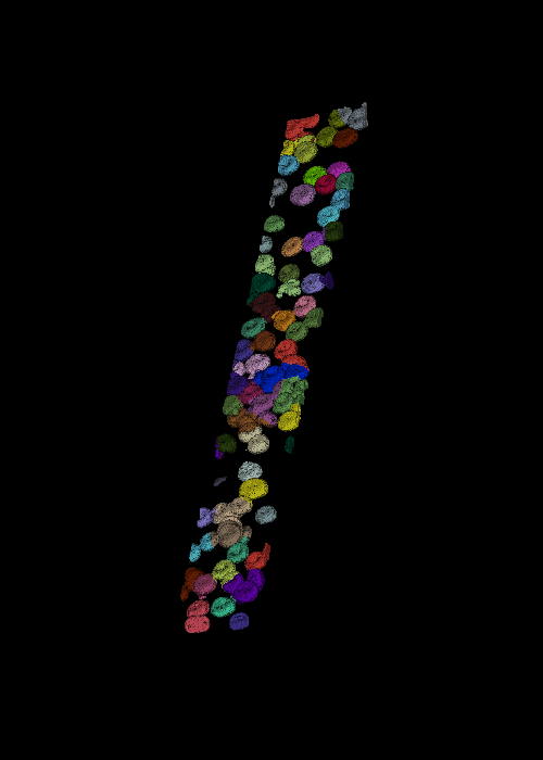
,time,channel,area,centroid-0,centroid-1,centroid-2,axis_major_length,axis_minor_length
0,T0,C0,49351.0,28.52,249.09,12.16,116.25,35.73
0,T0,C0,36859.0,18.90,353.81,23.41,89.78,25.56
0,T0,C0,35350.0,20.71,458.17,19.35,63.48,29.04
...

The label image and measurement table are written to your Save Directory when you run the save step from the Output tab.

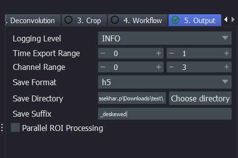
The Output tab is where you configure and run the final save. The other tabs (Deskew, Deconvolution, Crop, Workflow) only set up a preview; the Save button at the bottom of the plugin processes the full data set using all enabled tabs and writes it to disk.

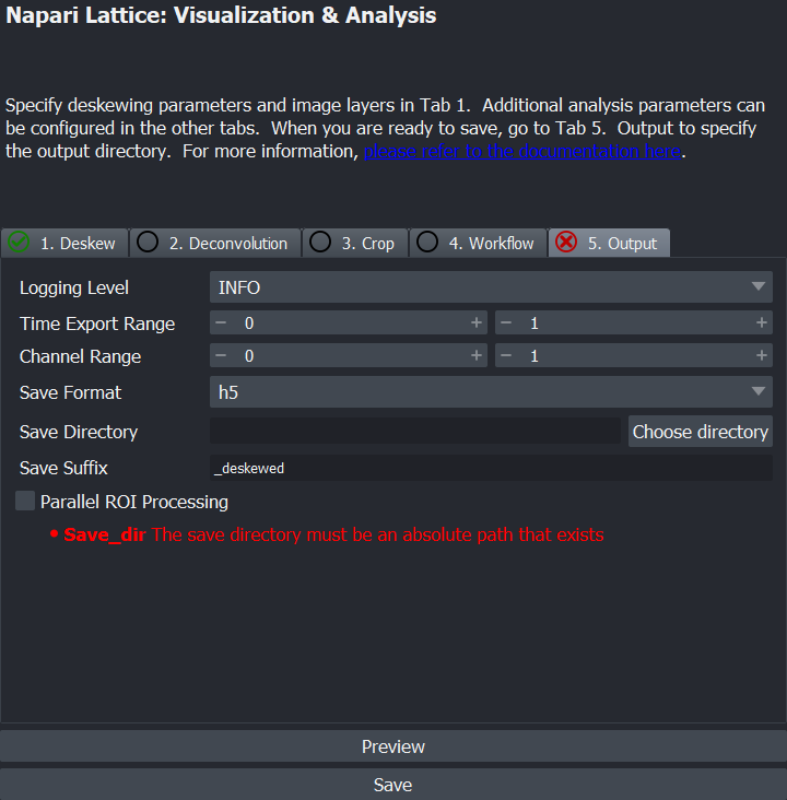
• Logging Level: verbosity of messages printed to the terminal (INFO is a good default; use DEBUG for troubleshooting).
• Time Export Range / Channel Range: the range of timepoints and channels to process and save. The maximum is set automatically from the loaded image.
• Save Format: the output file type.
  • tiff — a compressed OME-TIFF (.ome.tif)
  • h5 — HDF5 for BigDataViewer / BigStitcher
  • omezarr — OME-Zarr
• Save Directory: the folder the output files are written to.
• Save Suffix: appended to the output file name.
• Parallel ROI Processing: when cropping with multiple ROIs, process them in parallel worker processes. Leave this off while testing a single ROI. When on, set Workers to the number of processes, or 0 to let a memory-safe count be chosen automatically. See Parallel ROI Processing for details.

Once configured, click Save to run the pipeline and write the results to the chosen directory.

Multi-channel images

If you have multi-channel images and they are loaded as separate image layers, you multi-select them using Shift + Left Click.

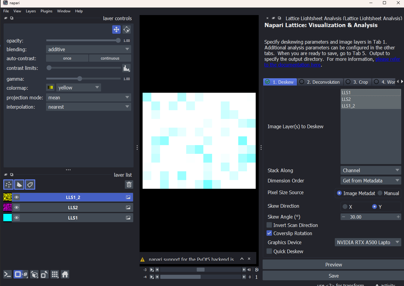
Make sure you enter the range of channels to be exported. This will only work if you've selected more than one channel.